Symbolic regression is a machine learning technique that finds a symbolic expression that matches data from an unknown function. In other words, it is a machinery able to identify an underlying mathematical expression that best describes a relationship between one or more variables.
The symbolic regression problem for mathematical functions has been tackled with a variety of methods, including:
Matlab
), gplearn (Python
);It builds a set of random formulas to represent the relationship between known independent variables and their dependent variable targets in order to predict them.
Each successive step (generation) of programs is then transformed (evolved) from the one that came before it (by selecting the fittest individuals) from the data (population) to undergo next (genetic) operations.
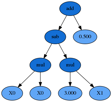
For example, to write the following expression:
\begin{equation} y = X^2_0 - 3 X_1 + 0.5 \end{equation}we can rewrite it as \begin{equation} y = X_0 \times X_0 - 3 \times X_1 + 0.5 . \end{equation}
But we can do more, we can use a LISP symbolic expression: \begin{equation} y = (+ ( - (\times X_0 X_0)(\times 3 X_1)) 0.5 ) \end{equation} or even, we can understand is as a syntax tree, where the interior nodes are the functions and the variables and constants are the terminal nodes:
It determines how well the program performs. As in other ML things, in GP we have to know whether the metric needs to be maximized or minimized in order to be able solve each specific problem:
Regression problems:
MSE
: mean squared error;RMSE
: root mean squared error;Classification problems:
LOG LOSS
: logarithmic loss;BIN CROSS-ENTROPY
: binary cross-entropy loss;Compreehends the parameters that should be chosen to perform the symbolic operation:
population_size
: number of programs competing in the first generation and every generation thereafter;function_set
: they are the available mathematical functions that you want to pass;generations
: the maximum number of steps until the programs stops;stopping_criteria
:it defines a default number meaning a perfect score $\Rightarrow$ used to stop the program too;p_crossover:
this crossover parameter is a percentage that takes the winner of a tournament and selects a random subtree from it to be replaced in the next generations;p_subtree_mutation
: it is a more agressive operation. It basically is another percentage parameter that allows to reintroduce extinct functions and operators into the population to maintain diversity;p_hoist_mutation
: another percentage parameter that is responsible to remove genetic material from tournament winners;p_point_mutation
: crazy percentage parameter $\Rightarrow$ it takes the winner of a tournament and selects random nodes from it to be replaced;max_samples:
increase the amount of subsampling performed on your data to get more diverse looks at individual programs from smaller portions of the data;parsimony_coefficient
: controls the penalty given to fitness measure during selection.gplearn
implements Genetic Programming in Python
, with a scikit-learn inspired and compatible API.
Here we will predict the Hublle evolution $H$ with the redshift $z$:
\begin{equation} H (z) = H_0 \sqrt{\Omega_k (1 + z)^2 + \Omega_m (1 + z)^3 + \Omega_r (1 + z)^4 + \Omega_{\Lambda}} \end{equation}where $H_0$ is the Hubble parameter, $\Omega_k$ is the curvature density, $\Omega_m$ is the matter density, $\Omega_r$ is the radiation density and $\Omega_{\Lambda}$ is the dark energy density of the Universe, all today.
import numpy as np
import pandas as pd
import matplotlib.pyplot as plt
from gplearn.genetic import SymbolicRegressor
import sklearn
from sklearn.ensemble import RandomForestRegressor
from sklearn.tree import DecisionTreeRegressor
from sympy import *
from sklearn.utils.random import check_random_state
import graphviz
import time
Initial dataset:
nsample = 1000
sig = 0.2
def Hz(z):
H0 = 67.3
Omega_m = 0.3115
Omega_r = 2.473*10**(-5)
Omega_de = 0.685
Omega_k = 1. - Omega_m - Omega_r - Omega_de
return H0*np.sqrt(Omega_k*(1 + z)**2 + Omega_m*(1 + z)**3 + Omega_r*(1 + z)**4 + Omega_de)
rng = check_random_state(0)
z = rng.uniform(0, 10, nsample)
H = Hz(z) + sig*np.random.normal(size=nsample)
data = np.array([z, H]).T
columns = ['z', 'H (z)']
df = pd.DataFrame(data = data, columns = columns)
df.head()
z | H (z) | |
---|---|---|
0 | 5.488135 | 624.287137 |
1 | 7.151894 | 876.945822 |
2 | 6.027634 | 702.550795 |
3 | 5.448832 | 618.878539 |
4 | 4.236548 | 454.219849 |
Data visualization:
plt.figure(dpi = 100)
plt.title('Huble parameter evolution')
plt.scatter(df['z'], df['H (z)'])
plt.ylabel(r'$H (z)$')
plt.xlabel(r'$z$')
Text(0.5, 0, '$z$')
X = df[['z']]
y = df['H (z)']
y_true = y
X_train, X_test, y_train, y_test = sklearn.model_selection.train_test_split(X, y, test_size=0.30, random_state=42)
X_train.shape, X_test.shape, y_train.shape, y_test.shape
((700, 1), (300, 1), (700,), (300,))
a) Choosing just some functions
function_set = ['add', 'sub', 'mul']
est_gp = SymbolicRegressor(population_size=5000,function_set=function_set,
generations=20, stopping_criteria=0.01,
p_crossover=0.7, p_subtree_mutation=0.1,
p_hoist_mutation=0.05, p_point_mutation=0.1,
max_samples=0.9, verbose=1,
parsimony_coefficient=0.01, random_state=0)
b) Fit:
t0 = time.time()
est_gp.fit(X_train, y_train)
print('Time to fit:', time.time() - t0, 'seconds')
| Population Average | Best Individual | ---- ------------------------- ------------------------------------------ ---------- Gen Length Fitness Length Fitness OOB Fitness Time Left 0 48.81 3.53838e+10 63 177.246 167.958 1.97m 1 51.35 187098 63 143.405 141.207 1.61m 2 63.31 197607 139 88.6634 83.3361 1.69m 3 80.92 3.82144e+06 139 87.1473 80.188 1.70m 4 73.40 1.7296e+06 143 85.3693 96.1901 1.51m 5 88.35 2.55467e+06 135 82.2406 83.0213 1.59m 6 123.16 6.42323e+09 129 58.0368 53.7706 1.70m 7 142.64 8.53495e+09 129 49.992 52.5158 1.73m 8 139.45 2.36822e+11 129 48.8323 44.3659 1.62m 9 135.79 2.364e+08 145 41.4034 45.2658 1.44m 10 132.55 7.76555e+07 149 40.9734 49.1365 1.31m 11 136.44 4.68113e+06 151 39.3009 36.933 1.19m 12 139.26 2.58968e+06 149 38.6996 42.3448 1.05m 13 150.45 2.31207e+07 119 30.0367 32.4589 56.88s 14 149.38 1.77535e+07 109 30.0065 32.7309 47.91s 15 148.63 3.0615e+11 139 27.309 29.4107 40.99s 16 153.20 7.27673e+06 139 26.9776 32.394 28.45s 17 146.20 1.45254e+09 125 23.7784 24.5737 18.87s 18 137.98 3.98801e+07 133 23.4379 26.5299 8.94s 19 139.36 3.7941e+09 147 19.6209 20.0325 0.00s Time to fit: 163.70209121704102 seconds
c) Prediction
t0 = time.time()
y_gp1 = est_gp.predict(X_test)
print('Time to predict:', time.time() - t0, 'seconds')
Time to predict: 0.003470182418823242 seconds
d) Score
score_gp1 = est_gp.score(X_test, y_test)
print('R2:', score_gp1)
R2: 0.9967157328344243
a) Equation
converter = {
'add': lambda x, y : x + y,
'sub': lambda x, y : x - y,
'mul': lambda x, y : x*y,
'div': lambda x, y : x/y,
'sqrt': lambda x : x**0.5,
'log': lambda x : log(x),
'abs': lambda x : abs(x),
'neg': lambda x : -x,
'inv': lambda x : 1/x,
'max': lambda x, y : max(x, y),
'min': lambda x, y : min(x, y),
'sin': lambda x : sin(x),
'cos': lambda x : cos(x),
'pow': lambda x, y : x**y,
}
next_e = sympify(str(est_gp._program), locals=converter)
next_e
b) Score
y_gp = est_gp.predict(X_test)
score_gp1 = est_gp.score(X_test, y_test)
score_gp1
0.9967157328344243
c) Plot
fig = plt.figure(constrained_layout=False, dpi=100)
gs = fig.add_gridspec(nrows=7, ncols=1)
f_ax1 = fig.add_subplot(gs[0:5,0])
plt.title('H (z) comparison')
plt.scatter(X_test, y_test, label = 'True function')
plt.scatter(X_test, y_gp1, marker = 'v', s = 10, label = 'Symbolic function')
plt.legend()
plt.ylabel('H (z)')
f_ax2 = fig.add_subplot(gs[5:7, 0])
plt.scatter(X_test, 1. - y_gp1/y_test, marker = 's', s = 10)
plt.ylabel('Residual')
plt.xlabel('z')
Text(0.5, 0, 'z')
d) Tree
dot_data = est_gp._program.export_graphviz()
graph = graphviz.Source(dot_data)
graph.render('images/ex1', format='png', cleanup=True)
graph
a) Don't imposing any function
est_gp = SymbolicRegressor(population_size=5000,
generations=20, stopping_criteria=0.01,
p_crossover=0.7, p_subtree_mutation=0.1,
p_hoist_mutation=0.05, p_point_mutation=0.1,
max_samples=0.9, verbose=1,
parsimony_coefficient=0.01, random_state=0)
b) Fit
t0 = time.time()
est_gp.fit(X_train, y_train)
print('Time to fit:', time.time() - t0, 'seconds')
| Population Average | Best Individual | ---- ------------------------- ------------------------------------------ ---------- Gen Length Fitness Length Fitness OOB Fitness Time Left 0 48.81 2.34608e+06 7 59.4318 66.2518 2.37m 1 50.93 11966.8 7 59.0484 69.7024 2.06m 2 58.86 5952.23 43 13.1229 14.6923 2.05m 3 58.18 9087.44 43 11.0273 12.0974 1.90m 4 62.73 11650.9 97 10.4827 10.7773 1.87m 5 75.55 9385.07 47 10.1926 11.7112 1.97m 6 56.27 6290.84 27 10.0121 13.1662 1.51m 7 49.54 8367.19 49 9.88528 12.5177 1.30m 8 41.17 14176.4 49 9.89063 12.4696 1.13m 9 36.73 5736.22 39 9.37762 7.83287 59.69s 10 33.50 15078.7 39 8.84874 12.5928 51.07s 11 32.06 2281.44 43 8.93255 11.8385 45.60s 12 35.45 1168.12 37 8.52854 10.3485 40.71s 13 42.58 891.934 77 8.13283 10.0993 37.35s 14 43.66 860.597 51 7.46917 8.47483 31.67s 15 44.09 674.422 51 7.35701 9.4842 25.23s 16 45.16 44730.3 55 7.17509 6.68837 19.05s 17 48.63 108859 57 6.87769 7.53629 13.35s 18 52.58 1407.36 49 6.37549 6.32367 6.75s 19 54.80 822.332 53 5.82337 5.21556 0.00s Time to fit: 132.9189989566803 seconds
c) Prediction
t0 = time.time()
y_gp2 = est_gp.predict(X_test)
print('Time to predict:', time.time() - t0, 'seconds')
Time to predict: 0.002447843551635742 seconds
d) Score
score_gp2 = est_gp.score(X_test, y_test)
print('R2:', score_gp2)
R2: 0.9995898043073126
a) Equation
next_e = sympify(str(est_gp._program), locals=converter)
next_e
b) Plot
fig = plt.figure(constrained_layout=False, dpi=100)
gs = fig.add_gridspec(nrows=7, ncols=1)
f_ax1 = fig.add_subplot(gs[0:5,0])
plt.title('H (z) comparison')
plt.scatter(X_test, y_test, label = 'True function')
plt.scatter(X_test, y_gp2, marker = 'v', s = 10, label = 'Symbolic function')
plt.legend()
plt.ylabel('H (z)')
f_ax2 = fig.add_subplot(gs[5:7, 0])
plt.scatter(X_test, 1. - y_gp2/y_test, marker = 's', s = 10)
plt.ylabel('Residual')
plt.xlabel('z')
Text(0.5, 0, 'z')
c) Tree
dot_data = est_gp._program.export_graphviz()
graph = graphviz.Source(dot_data)
graph.render('images/ex2', format='png', cleanup=True)
graph
a) Model and fit
est_tree = DecisionTreeRegressor(max_depth=5)
t0 = time.time()
est_tree.fit(X_train, y_train)
print('Time to fit:', time.time() - t0, 'seconds')
Time to fit: 0.014159202575683594 seconds
b) Prediction and score
t0 = time.time()
y_tree = est_tree.predict(X_test)
print('Time to predict:', time.time() - t0, 'seconds')
Time to predict: 0.0028460025787353516 seconds
#Score
score_tree = est_tree.score(X_test, y_test)
print('DT:', score_tree)
DT: 0.998831678221913
c) Plot
fig = plt.figure(constrained_layout=False, dpi=100)
gs = fig.add_gridspec(nrows=7, ncols=1)
f_ax1 = fig.add_subplot(gs[0:5,0])
plt.title('H (z) comparison')
plt.scatter(X_test, y_test, label = 'True function')
plt.scatter(X_test, y_tree, marker = 'v', s = 10, label = 'Decision Tree')
plt.legend()
plt.ylabel('H (z)')
f_ax2 = fig.add_subplot(gs[5:7, 0])
plt.scatter(X_test, 1. - y_tree/y_test, marker = 's', s = 10)
plt.ylabel('Residual')
plt.xlabel('z')
Text(0.5, 0, 'z')
a) Model and Fit
est_rf = RandomForestRegressor(n_estimators=100,max_depth=5)
t0 = time.time()
est_rf.fit(X_train, y_train)
print('Time to fit:', time.time() - t0, 'seconds')
Time to fit: 0.22199487686157227 seconds
b) Prediction and Score
t0 = time.time()
y_rf = est_rf.predict(X_test)
print('Time to predict:', time.time() - t0, 'seconds')
Time to predict: 0.023862361907958984 seconds
score_rf = est_rf.score(X_test, y_test)
print('RF:', score_rf)
RF: 0.9998512936885466
c) Plot
#Plot
fig = plt.figure(constrained_layout=False, dpi=100)
gs = fig.add_gridspec(nrows=7, ncols=1)
f_ax1 = fig.add_subplot(gs[0:5,0])
plt.title('H (z) comparison')
plt.scatter(X_test, y_test, label = 'True function')
plt.scatter(X_test, y_rf, marker = 'v', s = 10, label = 'Random Forest')
plt.legend()
plt.ylabel('H (z)')
f_ax2 = fig.add_subplot(gs[5:7, 0])
plt.scatter(X_test, 1. - y_rf/y_test, marker = 's', s = 10)
plt.ylabel('Residual')
plt.xlabel('z')
Text(0.5, 0, 'z')
fig = plt.figure(figsize=(12, 10))
for i, (y, score, title) in enumerate([(y_test, None, "Ground Truth"),
(y_gp, score_gp2, r"Symbolic Regressor: Score $= {:.4f}$".format(score_gp2)),
(y_tree, score_tree, r"DecisionTreeRegressor: Score $= {:.4f}$".format(score_tree)),
(y_rf, score_rf, r"RandomForestRegressor: $Score = {:.4f}$".format(score_rf))]):
ax = fig.add_subplot(2, 2, i+1)
points = ax.scatter(X, y_true, alpha=0.5)
test = ax.scatter(X_test,y, alpha=0.5)
plt.title(title)
The SymbolicClassifier works in exactly the same way as the SymbolicRegressor in how the evolution takes place. The only difference is that the output of the program is transformed through a sigmoid function in order to transform the numeric output into probabilities of each class.
In essence this means that a negative output of a function means that the program is predicting one class, and a positive output predicts the other.
from gplearn.genetic import SymbolicClassifier
from sklearn.datasets import load_boston
from sklearn.metrics import roc_auc_score
from sklearn.metrics import roc_curve
a) Loading:
from sklearn.datasets import load_breast_cancer
cancer = load_breast_cancer()
b) Description:
print(cancer.DESCR)
.. _breast_cancer_dataset: Breast cancer wisconsin (diagnostic) dataset -------------------------------------------- **Data Set Characteristics:** :Number of Instances: 569 :Number of Attributes: 30 numeric, predictive attributes and the class :Attribute Information: - radius (mean of distances from center to points on the perimeter) - texture (standard deviation of gray-scale values) - perimeter - area - smoothness (local variation in radius lengths) - compactness (perimeter^2 / area - 1.0) - concavity (severity of concave portions of the contour) - concave points (number of concave portions of the contour) - symmetry - fractal dimension ("coastline approximation" - 1) The mean, standard error, and "worst" or largest (mean of the three worst/largest values) of these features were computed for each image, resulting in 30 features. For instance, field 0 is Mean Radius, field 10 is Radius SE, field 20 is Worst Radius. - class: - WDBC-Malignant - WDBC-Benign :Summary Statistics: ===================================== ====== ====== Min Max ===================================== ====== ====== radius (mean): 6.981 28.11 texture (mean): 9.71 39.28 perimeter (mean): 43.79 188.5 area (mean): 143.5 2501.0 smoothness (mean): 0.053 0.163 compactness (mean): 0.019 0.345 concavity (mean): 0.0 0.427 concave points (mean): 0.0 0.201 symmetry (mean): 0.106 0.304 fractal dimension (mean): 0.05 0.097 radius (standard error): 0.112 2.873 texture (standard error): 0.36 4.885 perimeter (standard error): 0.757 21.98 area (standard error): 6.802 542.2 smoothness (standard error): 0.002 0.031 compactness (standard error): 0.002 0.135 concavity (standard error): 0.0 0.396 concave points (standard error): 0.0 0.053 symmetry (standard error): 0.008 0.079 fractal dimension (standard error): 0.001 0.03 radius (worst): 7.93 36.04 texture (worst): 12.02 49.54 perimeter (worst): 50.41 251.2 area (worst): 185.2 4254.0 smoothness (worst): 0.071 0.223 compactness (worst): 0.027 1.058 concavity (worst): 0.0 1.252 concave points (worst): 0.0 0.291 symmetry (worst): 0.156 0.664 fractal dimension (worst): 0.055 0.208 ===================================== ====== ====== :Missing Attribute Values: None :Class Distribution: 212 - Malignant, 357 - Benign :Creator: Dr. William H. Wolberg, W. Nick Street, Olvi L. Mangasarian :Donor: Nick Street :Date: November, 1995 This is a copy of UCI ML Breast Cancer Wisconsin (Diagnostic) datasets. https://goo.gl/U2Uwz2 Features are computed from a digitized image of a fine needle aspirate (FNA) of a breast mass. They describe characteristics of the cell nuclei present in the image. Separating plane described above was obtained using Multisurface Method-Tree (MSM-T) [K. P. Bennett, "Decision Tree Construction Via Linear Programming." Proceedings of the 4th Midwest Artificial Intelligence and Cognitive Science Society, pp. 97-101, 1992], a classification method which uses linear programming to construct a decision tree. Relevant features were selected using an exhaustive search in the space of 1-4 features and 1-3 separating planes. The actual linear program used to obtain the separating plane in the 3-dimensional space is that described in: [K. P. Bennett and O. L. Mangasarian: "Robust Linear Programming Discrimination of Two Linearly Inseparable Sets", Optimization Methods and Software 1, 1992, 23-34]. This database is also available through the UW CS ftp server: ftp ftp.cs.wisc.edu cd math-prog/cpo-dataset/machine-learn/WDBC/ .. topic:: References - W.N. Street, W.H. Wolberg and O.L. Mangasarian. Nuclear feature extraction for breast tumor diagnosis. IS&T/SPIE 1993 International Symposium on Electronic Imaging: Science and Technology, volume 1905, pages 861-870, San Jose, CA, 1993. - O.L. Mangasarian, W.N. Street and W.H. Wolberg. Breast cancer diagnosis and prognosis via linear programming. Operations Research, 43(4), pages 570-577, July-August 1995. - W.H. Wolberg, W.N. Street, and O.L. Mangasarian. Machine learning techniques to diagnose breast cancer from fine-needle aspirates. Cancer Letters 77 (1994) 163-171.
rng = check_random_state(0)
perm = rng.permutation(cancer.target.size)
cancer.data = cancer.data[perm]
cancer.target = cancer.target[perm]
X_train = cancer.data[:400]
y_train = cancer.target[:400]
X_test = cancer.data[400:]
y_test = cancer.target[400:]
X_train.shape, y_train.shape, X_test.shape, y_test.shape
((400, 30), (400,), (169, 30), (169,))
est = SymbolicClassifier(parsimony_coefficient=.01,
feature_names=cancer.feature_names,
random_state=1)
t0 = time.time()
est.fit(X_train, y_train)
print('Time to fit:', time.time() - t0, 'seconds')
Time to fit: 16.150514125823975 seconds
y_gpclas = est.predict_proba(X_test)[:,1]
y_gpclas.shape
(169,)
score = roc_auc_score(y_test, y_gpclas)
score
0.9693786982248521
a) ROC curve:
cutoff = 0.7
y_test_classes = np.zeros_like(y_test)
y_test_classes[y_test > cutoff] = 1
cutoff = 0.7
y_gpclas_classes = np.zeros_like(y_gpclas)
y_gpclas_classes[y_gpclas > cutoff] = 1
fpr, tpr, thresholds = roc_curve(y_test_classes, y_gpclas_classes)
plt.figure(dpi=100)
plt.plot(fpr, tpr, '-o', label = r'ROC curve ( area = {:.4})'.format(score))
plt.plot([0, 1], [0, 1], linestyle='--')
plt.xlabel('False Positive Rate')
plt.ylabel('True Positive Rate')
plt.title('ROC curve')
plt.legend()
<matplotlib.legend.Legend at 0x7f3e2e4cfdc0>
b) Tree:
dot_data = est._program.export_graphviz()
graph = graphviz.Source(dot_data)
graph